Introduction

A bit ago, I made a post about a result characterizing $k$-colorability of a graph using ring theory of ideals:

Thus graph coloring problem is reduced to an ideal membership problem. I think this result is cool for its own sake, but the next natural question is “does this make this problem any easier to solve?” I spent quite a bit of time seeing if I could make it work as a computational task, and this post is a sort of journal covering the hoops I had to jump through to try and make it feasible.

1. Smooth sailing

Disclaimer: this section covers mathematical background that I hope is accessible, but it is not strictly necessary to understand the implementation. At the end of the section, I outline the actual thing that needs to be computed, you may skip to it directly.

Here’s the nice thing. In general, to solve an ideal membership problem, we have to compute a Gröbner basis of said ideal. An ideal can be represented with many bases (generating sets), but some of them are much more amenable to doing any sort of computation, and Gröbner bases are the best of them. The downside is that computing such a basis is really hard by itself (at least as hard as graph coloring, for certain). The upside is that we don’t need to, and I will give a brief overview to explain this.

We begin with polynomial division. In a univariate polynomial ring, such as $\mathbb{R}[x]$, we have what is called the “division algorithm”: for any polynomials $f$ and $g$, we can find polynomials $q,r$ such that $f=qg+r$, where $\deg(r)<\deg(g)$, that is, we divide $f$ by $g$ with remainder. This works always because a univariate ring is a lovely and handsome Principal Ideal Domain, which means that any ideal $I$ can be generated by only one element, like $I=\langle x\rangle$; this is like how the set of even numbers in $\mathbb{Z}$ can be represented by $\langle 2\rangle$, i.e. all multiples of 2. But a multivariate ring, like $\mathbb{R}[x,y]$, does not have this property. So how do we divide polynomials in 2 variables?

When we divide $f$ by $g$, what we actually do is divide by the ideal $\langle g\rangle$. If you’ve taken any sort of abstract algebra, you may be familiar with this action as the canonical homomorphism $R\rightarrow R/\langle g\rangle$ sending each element of the ring to the coset of the ideal to which it belongs (the remainder is the coset representative). But in $\mathbb{R}[x,y]$, some (most) ideals are not principal; we have to write them as $I=\langle g_{1},g_{2}\rangle$. If you attempt to run the standard division algorithm to divide by $g_{1}$ and $g_{2}$ trying to find the quotients and the remainder in $f=q_{1}g_{1}+q_{2}g_{2}+r$, you may find that the order of $g_{1}$ and $g_{2}$ affects not only the quotients, but also the value of the remainder itself, so the “canonical homomorphism” is actually not a function at all.

A Gröbner basis is what lets us fix this, since their essential property is that they always produce the same minimal remainder $r$ when used as a divisor, regardless of the permutation of elements within. Thus we can actually compute $(f\mod I)$ when $I$ is expressed as a Gröbner basis $\langle g_{1},...,g_{n}\rangle$.

I haven’t really defined what constitutes a Gröbner basis, and actually I’m not gonna do that here at all, because the main takeaway that matters is that $I_{k}=\langle x_{i}^{k}-1\mid i\in[n]\rangle$ is already Gröbner. In particular, reducing a polynomial $f\mod I_{k}$ is simply reducing its every exponent mod $k$. Thus our problem is:

Examples

Before we begin, here are some examples of graphs and their corresponding polynomials, just to get a feel for it:

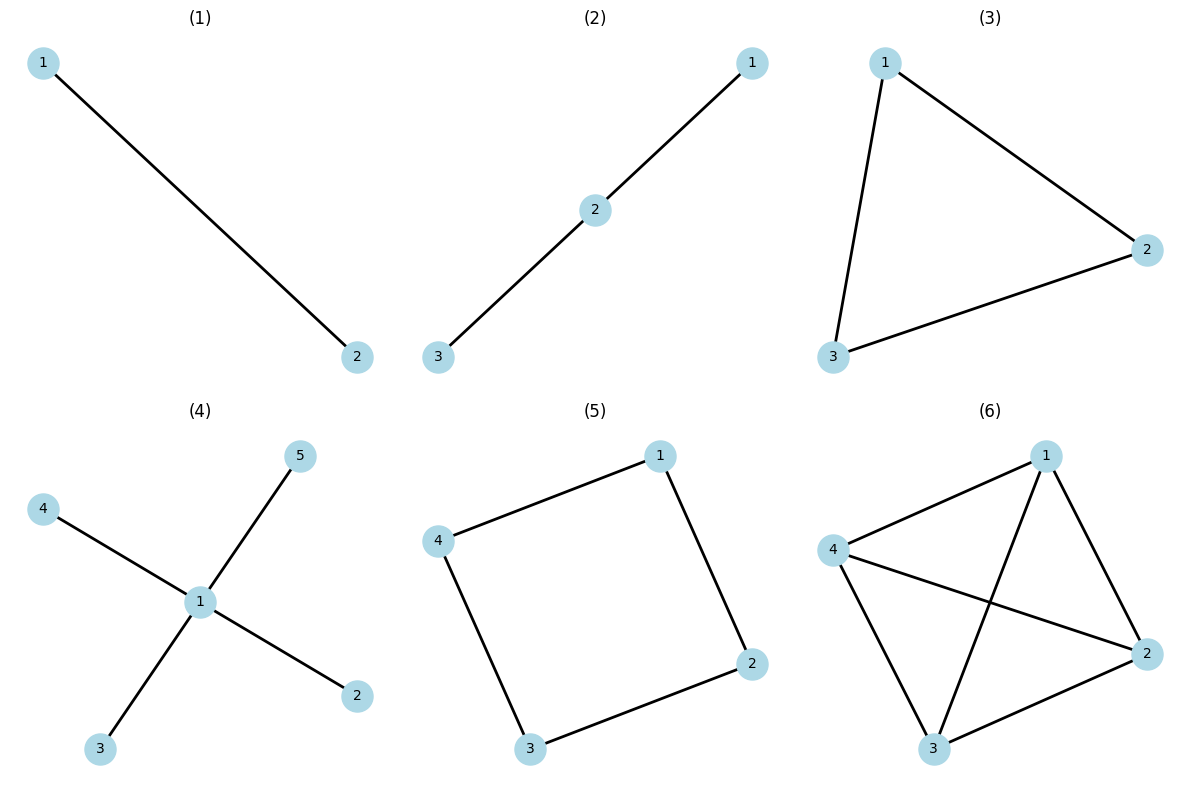
As you can see, these get large rather quickly.

2. The First Look

Since have a (theoretical, at this point) algorithm for checking whether $G$ is $k$-colorable, to find the minimum such $k$, or the chromatic number $\chi(G)$, we will simply run binary search; this works because is_colorable(G,k) is a monotonic function with respect to $k$.

def chromatic_number(G, k):
	low, high = 2, maxdegree(G)+1 # assume |E| > 0.
	med = (low+high)//2
	while low < high:
		bool k_valid = is_colorable(G, med)
		if k_valid:
			low, high = low, med
		else:
			low, high = med+1, high
	return med

This solves for $\chi(G)$ using $O(\log_{2}(\max\deg(G)-1))$ queries. We use $\max\deg(G)+1$ as that is the upper bound on $\chi(G)$ by Brooks’ theorem (and unless $G$ is $K_{n}$ or $C_{n}$ with $n$ odd, you can drop the +1). So going forward, all focus is on optimizing the query is_colorable.

The task therefore is repeated multiplication of $n$-variate polynomials. The main bottleneck here is storing and updating terms. My first choice here is processing the edges one by one and reducing exponents mod $k$ at each step, since that caps the number of possible terms to $k^{n}$ (an astronomical number, but at least it’s not unbounded). At each step we multiply the previous iteration of the polynomial $f_{t}$ by some $(x_{i}-x_{j})$:

f_0 = 1
for (i, j) in E:
	f_{t+1} = (f_t * x_i) - (f_t * x_j)
	f_{t+1} %= I_k

The second line in the loop reduces each exponent in each term mod $k$. A polynomial has the following expanded form:

We can represent it as a list of terms, each term consisting of a coefficient and a monomial, and each monomial is a list $[e_{1}^{(i)},...,e_{n}^{(i)}]$ of exponents for each $x_{j}$.

f_t = [
	(c1, [e11, e12, ..., e1n]),
	(c2, [e21, e22, ..., e2n]),
	...,
]

We multiply $f_{t}\cdot x_{j} \mod I_{k}$ by incrementing $j$th exponent in each term of $f_{t}$ (modulo $k$).

This is… less than ideal. First, while the updates themselves are fast, the memory footprint is atrocious, since we must allocate a vector for each term. Second, to simplify the polynomial (when we do the subtraction at each step), we want to combine like terms. To do this, we must iterate by pairs of terms in $f_{t}\cdot x_{i}$ and $f_{t}\cdot x_{j}$, which is $O(n^{2})$. Vector comparison is another $O(n)$ factor.

The natural two improvements are:

1. Hash the monomial exponent vectors into single integers for $O(1)$ comparison
2. Use a hashmap $\text{monomial exponent vector hash }\mapsto \text{ coefficient}$

exp_list = [
	(hash1, [e11, e12, ..., e1n]),
	(hash2, [e21, e22, ..., e2n]),
	...,
]

coeffs_map = {
	hash1 -> c1,
	hash2 -> c2,
	...
}

Now the algorithm can do this:

# input: edge ij, previous-step polynomial f_t
new_exps = []
new_coeffs = {}
for exp_hash, exp_vec in exp_list:
	exp_vec_i = copy(exp_vec)
	exp_vec_i = (exp_vec_i[i] + 1) % k
	new_hash_i = hash(exp_vec_i) # O(?)
	
	exp_vec_j = copy(exp_vec)
	exp_vec_j = (exp_vec_j[j] + 1) % k
	new_hash_j = hash(exp_vec_j)
	
	new_coeffs[new_hash_i] = coeffs[exp_hash]
	new_coeffs[new_hash_j] -= coeffs[exp_hash]
	new_exps.insert( (new_hash_i, exp_vec_i) )
	new_exps.insert( (new_hash_j, exp_vec_j) )
	
exp_list = new_exps
coeffs_map = new_coeffs

Okay, now assume hash() is constant time. This works nicely because combining like terms occurs naturally as we simply update coefficient values indexed by hashes of the exponent vectors. This doesn’t solve the storage problem, but the loop is certainly faster.

Okay, now un-assume hash() is constant time, because you cannot, in fact, process a length-$n$ vector in $O(1)$. You can do something else, though: make the hash incremental, i.e., homomorphic with respect to coordinate-wise incrementation, so we can compute new_hash_i from exp_hash and i in constant time. The rest of this section is dedicated to this problem.

There are two kinds of modifiable hashes that I considered for this: polynomial rolling hash and Zobrist hash. The former hashes a vector $A=[a_{1},...,a_{n}]$ as

where $B$ and $P$ are pre-determined (prime) constants. This hash is widely used in competitive programming for processing strings, since it has nice properties for when you want to compare prefixes and suffixes. For our purposes, defining $A'$ to be the vector identical to $A$ except in the $j$th coordinate, for which the value is $b\neq a_{j}$, we write:

So we undo the $j$th coordinate in the original hash and replace it with the desired value $b$, which in our case would be $a_{j}+1 \mod k$.

The Zobrist hash is quite different; it is incremental by design and was invented to store games like chess - when a move is made, the state of the board changes only slightly, and you’d not want to recompute the hash from scratch when only two squares change.

Generate a $n\times k$ table of random values, call it $Z$. Define

where $\oplus$ is bitwise XOR. Now to modify the $j$th coordinate, we again undo the current value and replace it with another:

Both of these hashes work, but for this task I went with Zobrist, since it doesn’t require finding suitable constants, XOR is faster than mod-multiplication, and overall it’s just cleaner.

An aside about benchmarking

When I began this project, I wanted to put together some graphs for testing accuracy and speed. Initially I drew a few up by hand, and tested my results against the symbolic computation done by SageMath. For a graph on more than $10$ vertices, SageMath took too long, though, and I didn’t want to generate random graphs and run actually practical coloring algorithms on them to figure out the true $\chi(G)$. For this reason I turned to two known graph families: the Mycielski and the Turán graphs. The point is that both of them are easily constructible and have a regular structure that makes the chromatic number a fundamental property, without needing any computation.

The Mycielski graph $M_{k}$ is specifically designed to have chromatic number $k$, with each successive $M_{k}$ being constructed iteratively from $M_{k-1}$. The special property is that it has no triangle subgraphs, making it quite sparse. The Turán graph $T_{n,r}$ is the opposite - it is the $r$-partite complete graph, having chromatic number $r$ and as many edges as possible.

3. Eliminating Exponent Vector Storage

The Zobrist hash trick allows us to compare monomials’ exponent vectors via their hashes, as well as update these hashes incrementally. However, the memory footprint remains: to update a hash by incrementing $a_{j}$, we actually have to know the current value, because the value we set is $a_{j}+1$ if $a_{j} < k$ and $0$ otherwise; there is a branch involved. We cannot perform a “blind” incrementation mod $k$ on the hash, so we must store the entire vector.

This was a glaring inefficiency that didn’t let me sleep at night for some time.

Okay, so the “blind” wrap-around mod $k$ should point to a cyclic representation of some kind. Suppose $G$ is a group of prime order $p$, so every non-identity element is a generator. If we pick $n$ such elements $g_{1},...,g_{n}$ and define $h(A)=\prod_{i\in n}g_{i}^{a_{i}}$, then we will see that we can change the $j$th element to some arbitrary element $b$ with:

This idea I found in Bellare et al. (2021)¹. The group here would be a multiplicative group mod $p$, where $p$ is be chosen to satisfy $p=2q+1$ for another prime $q$; this ensures $\mathbb{Z}_{p}^{\times}$ has prime order. However, this does not yet give us the cyclic effect mod $k$. For that, we can use a trick: choose $p$ to instead satisfy $p\equiv 1\pmod k$. Since it no longer has prime order, not every element is a generator, but nevertheless there are $\varphi(p-1)$ of them². We need $n$ elements $g_{1},...,g_{n}$ with order $k$, for which we can take a generator $g$ and raise it to power $(p-1)/k$. Once again let $h(A)=\prod_{i\in[n]}g_{i}^{a_{i}}$ but now, to increment the $j$th coordinate we simply multiply $h(A')=h(A)\cdot g_{j}$. This works because we’ve made it so $g_{j}^{k}=e$, which gives us the desired modulo effect.

However, there’s a significant problem with this approach (see if you can find it). Because we take a product over elements with $g_{i}^{k}=e$, the set of outputs is exactly the elements of the group which satisfy this. So what is the size of our hash’s image?

So while the hash function thus constructed satisfies our original requirements, it can only ever output $k$ distinct values… This is far too few to ever be useful. My solution here was to extend this idea - rather than have only one $k$-cyclic subgroup which hard-caps our outputs to a small number, we embed multiple.

Let $p$ and $q$ be prime, and $N:=pq$. Recall that $\mathbb{Z}^{\times}_{N}\cong \mathbb{Z}^{\times}_{p}\times \mathbb{Z}^{\times}_{q}$ and that each of the groups on the right side are cyclic. Choosing again $p$ such that $|\mathbb{Z}^{\times}_{p} |=p-1$ is divisible by $k$, we guarantee the group contains a cyclic subgroup of order $k$ (isomorphic to the cyclic group $C_{k}$). We choose $q$ likewise, with the only added constraint of $p\neq q$. Applying the isomorphism above, we’ve ensured that $C_{k}\times C_{k}$ is isomorphic to a subgroup of $\mathbb{Z}_{N}^{\times}$. If $\langle g\rangle=C_{k}$, then $C_{k}^{2}=C_{k} \times C_{k}=\langle (g,e), (e,g)\rangle$. In other words, if we can find the elements corresponding to $(g,e)$ and $(e,g)$ in $\mathbb{Z}_{N}^{\times}$, we can add an extra dimension to our hash image!

Let’s do this concretely. The Chinese Remainder theorem gives us $\mathbb{Z}^{\times}_{p}\times \mathbb{Z}^{\times}_{q}\cong \mathbb{Z}^{\times}_{N}$, let $\phi$ be this isomorphism, and suppose we’ve found the elements $h_{p}\in\mathbb{Z}^{\times}_{q}$ and $h_{q}\in\mathbb{Z}^{\times}_{q}$ as above, so the $\text{ord}(h)=k$. The basis $\set{ (h_{p},e),(e,h_{q})}$ generates $C_{k}^{2}$ and we can lift it to $\mathbb{Z}^{\times}_{N}$: define $g_{1}:=\phi(h_{p},e)$ and $g_{2}:=\phi(e,h_{q})$. Restating above, we get:

The point is that the size of $\text{span}\set{g_{1},g_{2}}$ in $\mathbb{Z}^{\times}_{N}$ is $k^{2}$ and we can find these elements very easily using a CRT solver (essentially the implementation of $\phi$) for the systems

Lastly, we choose $s_{1},s_{2}$ from $0,...,k-1$ randomly, and define $w=g_{1}^{s_{1}}g_{2}^{s_{2}}$. Since $g_{i}^{k}=e$, we know also that $w^{k}=e$. Now rather than just one, generate $n$ pairs $(s_{1}^{(i)},s_{2}^{(i)})$, and for each of them let $w_{i}$ be defined likewise. What we have done at this point is construct $w_{1},...,w_{n}\in \mathbb{Z}^{\times}_{N}$ which span the product cyclic subgroup and satisfy $w^{k}=e$, which is the exact condition we wanted. We formalize the hash function for $A=[a_{1},...,a_{n}]$ as

and verify that for $A'$ defined as $A$ but with $j$th coordinate incremented mod $k$, it satisfies

The order of each $w$ is $k$ (or, in rare cases, a divisor of $k$ if $gcd(k,s_{1},s_{2})>1$), so $w^{k}$ cycles back to $e$, and $\text{span}\set{w_{1},...,w_{n}}=\text{span}\set{g_{1},g_{2}}$ with size $k^{2}$. Thus we have our magic hash!

Asterisks

This yields a hash with image size $k^{2}$ but in practice this is still far too small. However, this method is entirely extendable: rather than use two primes, we use $N:=p_{1}p_{2}...p_{d}$, leverage $\mathbb{Z}_{p_{1}}^{\times}\times ... \times \mathbb{Z}_{p_{d}}^{\times}\cong \mathbb{Z}_{N}^{\times}$ and the generalization

to make $w_{1},...,w_{n}$ span $d$ dimensions, resulting in the image size $k^{d}$. Since the operations in $\mathbb{Z}_{N}^{\times}$ happen modulo $N$, this is the bottleneck - the product of our $d$ distinct special primes must fit in an (128-bit) integer data type. To maximize $d$, we choose the primes to be as small as possible, but on average, we can get $\approx 18$. Still, this gives us a very sizable output space.

A key step I’ve skipped is producing a generator $g$ of $\mathbb{Z}_{p}^{\times}$. There’s not a known closed form solution for this problem, but (for any $p$) on average about a third of the elements of $\mathbb{Z}_{p}^{\times}$ are generators, so a guess-and-check algorithm is actually quite efficient for this. We know by Lagrange’s theorem that if an element $g$ has order $m < n:=p-1=|\mathbb{Z}_{p}^{\times}|$, then $m$ is a divisor of $n$. The contrapositive tells us that if for some $m\mid n,\; g^{m}=e$, then $g$ is not a generator; thus, we will pick a random element and go through all maximal divisors of $n$ to see if our candidate evaluates to $e$ with that exponent; if it doesn’t for any of them, we’ll have found our generator.

while True:
	x = randint(2,p-1)
	failed = False
	for q in prime_factors(n):
		if pow(x, n/q, p) == 1:
			failed = True
			break
	if not failed:
		return x
	

For prime factorization I will precompute the SPF array (spf[n] = smallest prime factor of n) up to a constant maximum; this needs only to be done once and allows $O(\log x)$ factorization. I use this method very often in competitive programming.

Now having found the generator of each $\mathbb{Z}_{p_{i}}^{\times}$, we let $h_{i}$ be it’s $((p_{i}-1)/k)^{\text{th}}$ power; observe that each $h_{i}$ has order $k$ and thus $C_{k}\cong \langle h_{i}\rangle \leq \mathbb{Z}_{p_{i}}^{\times}$.

Summary

To recap, what we’ve done so far is construct a group $\mathbb{Z}_{N}^{\times}$ that contains as many embedded copies of the cyclic group $C_{k}$ in it as we could fit. We know that their product $C_{k}\times ... \times C_{k}\cong \langle h_{i}\rangle\times...\times\langle h_{d}\rangle$ is a group to which there exists an isomorphic subgroup in $\mathbb{Z}_{N}^{\times}$ by the Chinese remainder theorem. We find the vectors spanning $C_{k}^{d}$ and lift them to $\mathbb{Z}_{N}^{\times}$, and we generate weights which give us the cyclic incrementation property.

As a final note, solving a CRT modular system of $d$ equations in the standard way requires $O(d)$ time; as there are $d$ such systems, we’re looking at $O(d^{2})$. However, the systems are all vectors of the “standard basis”: in the $i$th vector, all elements but the $i$th are identity. We can use this to speed up the computation to $O(d)$ in total by doing it in a batch with $O(1)$ per system/vector with $N$ known.

4. Reduction via Edge Ordering

The algorithm can be viewed as a process that begins with an empty graph on $n$ vertices and adds an edge at each step. The revelation of each edge $(ij)$ corresponds to multiplying the previous step’s polynomial by $(x_{i}-x_{j})$. The number of terms in this polynomial grows very quickly (more or less exponentially, as you might imagine); the more terms we have at step $t$, the more we will have to process and insert at $t+1$. But not all edges give the same growth. Can we slow the term count growth by revealing edges in a clever order?

The answer is yes, and here’s a simple example: $f_{t}$ is the polynomial of the partial graph with edges $1,...,t$ (with respect to a particular ordering), and $\text{T}(f_{t})$ is the number of terms in the polynomial. Notice that the second ordering produces fewer terms at steps 3 and 4. Of course, the final result will be the same in any ordering as the final graph is fixed, but smaller intermediate results means less work at each subsequent step.

Here’s a more noticeable difference: The second ordering processes, in total, 73 fewer terms than the first. Clearly, among all orderings of edges of the graph $G$, there must be an ordering which yields the fewest intermediate terms over the course of execution. So… what is it?

This is a hard problem, I hate to say, and I don’t have a solution. But there are some heuristics which can give a pretty good approximation. The main problem is the behavior of the function $\text{T}(\cdot)$ - I don’t have a simpler formula for the term count than its definition, even a recurrent one. However, observe that each time we introduce an edge containing an endpoint not already in the graph, the term count doubles. This should make sense: in the step $f_{t}\mapsto x_{i}f_{t}-x_{j}f_{t}$ the terms of our polynomial are duplicated, but a cancellation may occur when we combine like terms. However, if $x_{i}$ or $x_{j}$ is not in $f_{t}$ already, a term from $x_{i}f_{t}$ can never be equal to a term in $x_{j}f_{t}$. Thus, $\text{T}(f_{t+1})\leq2\text{T}(f_{t})$ with equality iff $x_{i}$ or $x_{j}$ are added for the first time. In a way, our task here is to maximize cancellation, which occurs when we link two vertices already connected; that is, close a cycle.

Here’s the key to why the second ordering in the both above examples wins: we close cycles greedily, aiming to close the shortest cycle available at each step, as short cycles provide the largest cancellation effect. When no cycles can be closed immediately, we attempt to predict which vertex reveals would produce potential for shortest cycles in the future. This method allows us to maximize cancellation at each step, and thus reduce the number of intermediate terms.

Let’s denote $G_{t}$ as the partial graph with the first $t$ edges revealed. Which edge should we pick next to maximize the closure of shortest cycles? A working strategy is to compute the distances $d_{t}(u,v)$ for all edges $uv$ remaining not revealed at step $t$ and pick the one that minimizes this distance, thereby closing a $d_{t}(u,v)+1$-long cycle. Naively this would require recomputing the distances in $G_{t}$ between the endpoints of all potential edges at every step; with BFS it comes out to $O((m+n)m^{2})$ where $m$ is the number of edges in $G$. Here, there’s a clever trick we can do: observe that if we insert an edge $uv$, the distance between any two other vertices $x$ and $y$ changes in a very predictable way.

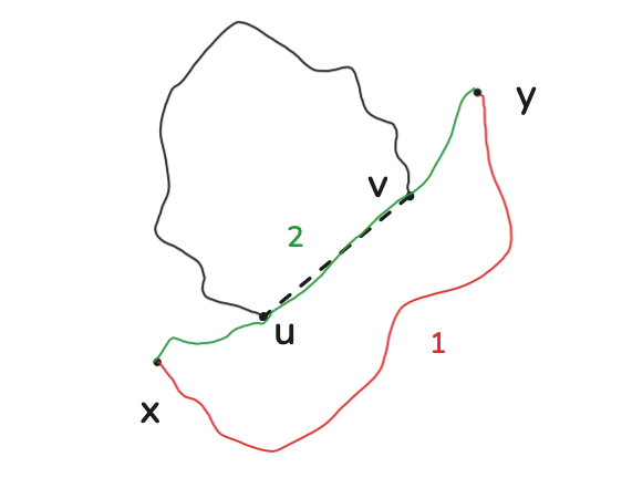
Here we plan to reveal the edge $uv$ and the black solid line is the shortest path between $u$ and $v$ in $G_{t}$ (prior to the insertion). What is the shortest path between $x$ and $y$ in $G_{t+1}$? There are two options: it either does not include the edge $uv$ at all (1) or includes it once (2). In the first case, $d_{t+1}(x,y)=d_{t}(x,y)$, and in the second, the route first takes the segment $x-u$, then the newly added shortcut edge, then the segment $v-y$, so $d_{t+1}(x,y)=d_{t}(x,u)+1+d_{t}(v,y)$. We also get a candidate path by swapping $u$ and $v$ in this expression. Thus, to update distances after the insertion of $uv$ we write:

We still need to know the distances to $u$ and $v$, so we will run BFS to get them. The algorithm looks like this and runs in $O((n+m)m)$:

order = []
future_edges = edges
d = {{a,b} : INF for {a,b} in edges} # distances map for future edges
while future_edges not empty:
	if have_finite_distance: # can close a cycle
		# take shortest distance edge
		uv = min(future_edges, key=d)
		future_edges.delete(uv)
		order.append(uv)
		
		u_dists = bfs(u)
		v_dsists = bfs(v)
		
		# update remaining distances
		for xy in future_edges:
			d[xy] = min(d[xy], u_dists[x]+1+v_dists[y], u_dists[y]+1+v_dists[x])
			if d[xy] < INF:
				have_finite_distance = True
	
	else:
		# ...

We want to defer the revealing of new vertices (revealing edges with a previously unseen endpoint) and prioritize adding edges between vertices already present. But If all distances on future edges are infinite, we can no longer close a cycle, so we must extend our graph to a new vertex. This cannot be done greedily and requires a certain prescience - it’s not clear which new vertex will lead to short cycles in the future. A heuristic can be used here: pick the vertex with the most back-edges to the discovered subgraph. The edge will be taken arbitrarily (though this can also be improved):

future_vertices = vertices
revealed_neighbors = {v : 0 for v in vertices}
	# ...
	else:
		v = max(future_vertices, key=revealed_neighbors)
		future_vertices.delete(v)
		# update futures and pick arbitrary back-edge from v
		for w in G.neighbors(v):
			if w not in future_vertices:
				u = w
			revealed_neighbors[w]++
		order.append(uv)

This is not an exact solution to the ordering problem, but it performs decently well for slowing down growth of terms. Unfortunately, since every new vertex reveal doubles the term count with no chance for cancellation, we’re still looking at $\geq 2^{n}$ terms in the expression.

5. A Faster Mod-Multiplication

At this point, the algorithm clears Mycielski $M_{4}$ in a fraction of a second, but struggles to make it past the first ~25 edges of $M_{5}$. A closer look at performance reveals that over a third of the CPU cycles are spent on doing mod-multiplication to update the term hash entries. And no wonder, since my algorithm for doing that up to this point looks like this:

ui128 modmult(ui128 a, ui128 b, ui128 m) 
{
	ui128 result = 0;
	while (b>0) {
		if (b&1) 
			// result = (result + a) % m;
			result=(result>=m-a) ? result-(m-a) : reuslt + a
		//a = 2*a % m;
		a = (a>=m-a) ? a-(m-a) : 2*a;
		b >>= 1;
	}
	return result;
}

This is awful and is essentially naive multiplication through addition in $O(\log b)$. The reason I did this initially was because 128-bit ints are the largest int data type in C++, so I could not cast the intermediate result $a\cdot b$ (which is up to 256 bits) to a larger type before taking mod. This was my next challenge.

Fortunately for me, some clever people solved this problem back in the 80s. The method I went for is called Montgomery multiplication. I won’t go into the full detail; I think the Wikipedia page explains it really well, it’s what I used to learn it. The base concept is this: we pick a radix base $r$ to be coprime to $m$, find the special Montgomery form $a*b$ defined in relation to $m$ and $r$, and express our result as $x\equiv (a*b)r^{-1}\pmod m$. To find the remainder in constant time, we must use the division operation which is the most expensive arithmetic instruction; what this lets us do is push the division over to $r$ rather than an expression of $a$ or $b$. The twist here is that we pick $r$ to be a power of two, which makes division as simple as bit shifting.

Montgomery speeds up my modmult by a factor of ~x15, from 0.00414 to 0.00026ms on average for 128-bit ints.

6. Last ditch efforts

The Monty optimization pushes my CPU time spent on modmult down to about 5%; most of the rest is the time spent on the methods of unordered_map - allocation, the []get operator, emplace, and a couple minor ones. My guess is that at this point the fault is in frequent cache misses - the STL hashmap allocates nodes on the heap scattered across memory. I switched to a flat, open addressing map from the GTL library developed by Gregory Popovitch. It actually has a pretty cool parallel hashmap template that breaks the map into 16 submaps and leverages SIMD instructions to speed up search and resizing; however, it turned out that for my use case the standard flat map was faster. I attribute this to my never needing to resize - I reserve sufficient space at initialization.

Open addressing gives a nice bonus, but with all these optimizations I could not break Mycielski $M_{5}$ (23 vertices, 71 edges) or Turán $T_{15,3}$ (15 vertices, 75 edges). The space footprint still grows exponentially, and by 30-35 edges in my CPU begins stalling as most time is spent waiting for memory rather than actual computation.

A strange trick I discovered here: it turned out that the map<ui128, int> was considerably slower than map<ui128, int64_t> - running on $M_{5}$, the first 30 edges took about 20% less time to process. Initially I guessed this is due to memory alignment rules splitting the 20-byte pairs across different 64-byte memory segments, requiring two cache lines to get a single pair; but in hindsight I don’t believe this is right - both options should require a full 32 bytes with padding to store. This is something I might investigate further.

Another idea I spent considerable time on: one could discard the hashmap entirely and switch to simple vectors. The problem requires us to match terms with equal monomial hashes, so if $x_{i}f_{t}$ and $x_{j}f_{t}$ were both represented by sorted arrays, we could do a zip merge to combine them into one. This would have a benefit over the hashmap since it would give us better locality control and improve the cache hit rate. However, sorting the arrays would take a long time (I tried with radix sort, it’s theoretically $O(n)$ but still slower than the hashmap approach), so instead what would be nice to have is a sort order that would be invariant under the action of multiplying each element by $w_{j}$. That is, if $h_{1}\prec ... \prec h_{T}$ is the sorted array of hashes of terms of $f_{t}$, then for $x_{i}f_{t}$ we maintain $h_{1}w_{i}\prec ...\prec h_{T}w_{i}$ and likewise for $j$. Then we could simply perform a sorted merge. The problem is, such a total order is impossible in a finite group: suppose elements of $G$ are ordered as $g_{1}\prec ... \prec g_{n}$ and we scale by $w\in G\text{ with }w\neq e$, then $wg_{1}\neq g_{1}$ is out of order.

However, I’m not entirely convinced. For one, our condition is slightly weaker than this: not all elements can appear as $w$ and they are known in advance. For another, we don’t need to have a linear order - we could use a circular one. A circular order on a set $S$ is a trinary relation $[a,b,c]$ that indicates the order in which you’d see elements moving along the circle. For instance, if $S$ are hours of the clock, $[1,4,9]$ is true but $[4,8,5]$ is not. One could imagine the list of terms as a circular array (first and last elements are considered adjacent) sorted under a circular ordering, so a sorted merge could work much the same way.

Conclusion

Ultimately, there’re many things left I could still investigate to improve performance, from high level mathematical representation to hardware optimization. This was an interesting experiment, and though I’ve learned some things I had not expected to even touch on, the practical results are… meager - this method only works for very small graphs. I wouldn’t recommend it.

7. Verdict

If you need a graph colored, I advise using something less deranged.